Follow these steps to compare two columns in Excel.
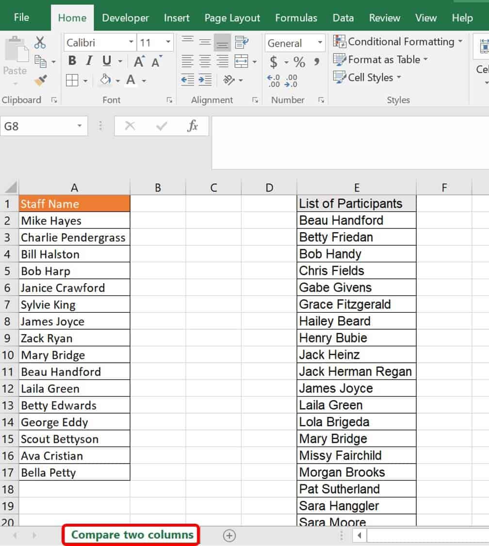
You’ll see a list of staff members in a department. In this example, you want to compare these names to the list of participants from your company’s annual field day to determine who you need to thank for their help. We have a List of Participants column and a separate list of employees in the department on the worksheet. The lists don’t necessarily need to be on the same worksheet, but for visualization purposes, we placed them here. As noted above, you could also perform the search by referring to a list in another worksheet or workbook; just follow the syntax for these functions above.
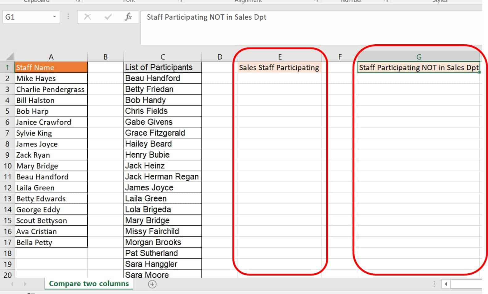
In this example, label the extra columns Sales Staff Participating and Participants NOT in Sales Dpt. The first extra column is for the values duplicated in the two columns, and the second is for identifying the unique values in column C (those who participated, but are not members of the sales department).
*=VLOOKUP(A2,C:C,1,FALSE)*
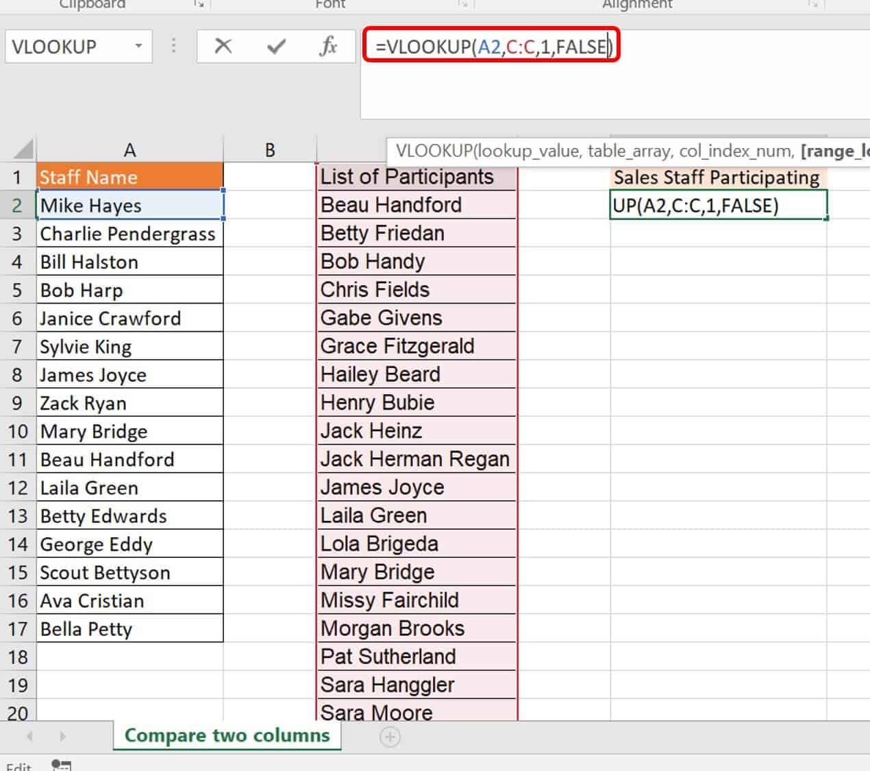
Breaking down this formula:
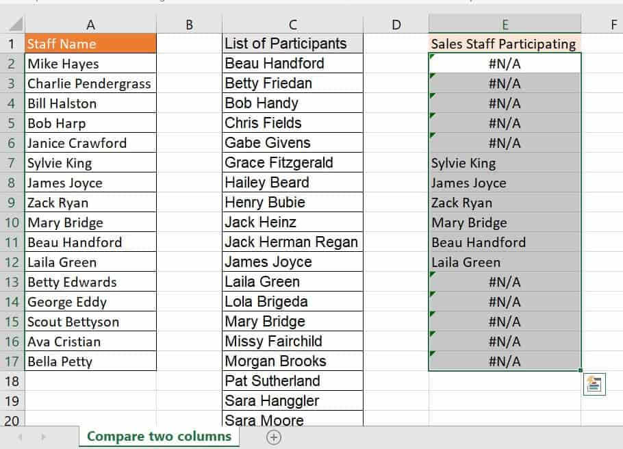
As you can see, the staff that participated in field day showed up by name in column E. The remainder of your sales staff elicited a #N/A error because their names were not listed as participants in column C.
In the above example, you compared two lists to find an overlap. This option provides the data you need, but also gives you #N/A errors where the data does not overlap. As an Excel expert, you know this means that your formula was successful. However, other people looking at this may think #N/A means something is wrong.
For a better-looking list, you can mask the #N/A errors by wrapping your VLOOKUP formula with an IFERROR function.