Author: Alphaist
In this article, we will try to understand Loss versus Rebalancing which is currently the most important issue in the DEX. Before we begin We’d like to ask you one quiz first. Suppose you bought Apple stock yesterday for $100 and were able to sell it for $110. Was this a good deal? Most people would probably say it was a good deal.
But is it really? Now suppose the S&P 500 ETF had risen from $100 to $120 in the same period. Your investment has not produced a return below the market average. If your reason for investing is purely in Apple itself, no problem, but if your goal is to maximize your own portfolio value, you should have bought an ETF in the S&P 500. Of course, this is a bit of a strong assumption since it is based on a single day, but if you have the same situation over a longer period of time, you may have profited in absolute dollars, but in relative terms you have lost an opportunity for further gains.
Something similar occurs with liquidity provision in the DEX. The concept of ‘Loss versus Rebalancing’ can be viewed as a transfer of value outside the application, stemming from the information asymmetry between the informed trader and the liquidity provider. On the other hand, it serves as a useful indicator for comparing the opportunity losses between the Rebalancing Portfolio and the Liquidity Provider’s portfolio. This means you can assess whether you’re taking on the market’s risk or the inherent risk of the Liquidity Provider (LP) when offering liquidity. Suppose you’ve made a 10% return on your liquidity offering. You can now evaluate whether this transaction is advantageous or not, in the context just described.
Loss versus Rebalancing is a measure of the LP of an AMM based on a paper published in August 2022 by Jason Milionis, Ciamac Moallemi, Tim Roughgarden, and Anthony Lee Zhang. The paper contains very advanced mathematical content, including stochastic process theory and the Black-Scholes model, which may be difficult for many DeFi users to understand.
In this article, we will try to make such content understandable to many readers by applying specific numerical values and supplementing the mathematical formulas. We will start with a simple example to help you better understand Loss versus Rebalancing, and then add more detailed explanations towards the bottom of the article.
Now, as an example, let’s consider providing liquidity to UniswapV2. You provide liquidity of 1 ETH and 1000 USDC or a total of $2000, when 1ETH = 1000USDC at t = 0. On the other hand you hold an additional 1 ETH and 1000 USDC. Note that the Rebalancing Portfolio is based on the CEX price for buying and selling assets. Also note that the Rebalancing Portfolio has nothing to do with rebalancing, which may be thought of as changing the price range for providing liquidity in a DEX with concentrated liquidity, such as Uniswap V3.
Let’s use an example to illustrate liquidity provision in UniswapV2. Imagine you’re providing liquidity with 1 ETH and 1000 USDC, which totals $2000 at the initial time, 1ETH = 1000USDC at t = 0. In addition to this, you also hold another set of assets comprising 1 ETH and 1000 USDC separately. It’s important to note that the ‘Rebalancing Portfolio’, in this context, refers to the strategy of buying and selling assets based on the Centralized Exchange (CEX) prices. Also, it’s crucial to understand that this Rebalancing Portfolio is distinct from the concept of ‘rebalancing’ in the context of a Decentralized Exchange (DEX) with concentrated liquidity, like Uniswap V3. In the latter case, ‘rebalancing’ typically involves adjusting the price range for providing liquidity.
Now suppose that 1ETH = 4000USDC at t = 1. In this case, LP’s portfolio will be composed of 0.5 ETH and 2000 USDC according to the formula x*y=k. Portfolio Value will be 0.5ETH * 4000USDC + 2000USDC which is $4000.
Now consider the composition of the Rebalancing Portfolio. As mentioned earlier, the Rebalancing Portfolio always rebalances at the CEX price. Therefore, let us assume that the Rebalancing Portfolio is composed of 1 ETH and $1000 USD, and given that 1 ETH is $4000 USD, 1ETH * 4000USDC + 1000USDC = 50000USDC. In other words, compared to the LP portfolio, we have gained $1000 more relative to the LP portfolio. Many people think that this is the same indicator as Imparment Loss. It is true that they are the same up to this point, but this is where we can understand the difference between the two.
Suppose that 1ETH = 1000USDC again at t = 2.In this case, IL is 0. However, the LVR is different, because LP’s portfolio will again consist of 1 ETH and 1000 USDC. Therefore, the Portfolio Value is 1ETH * 1000USDC + 1000USDC, which is $2000. The Rebalancing Portfolio on the other hand is 1ETH * 4000USDC + 1000USDC, but to duplicate the LP portfolio mentioned earlier, it will be rebalanced to 0.5ETH * 4000USDC + 3000USDC. And the current price of ETH is 0.5ETH * 1000USDC + 3000USDC = 3500USDC since 1ETH = 1000USDC.
If we rebalance again at the CEX price 1ETH + 2500USDC. We have prevented a loss of $500 relative to the LP portfolio. The Imparment Loss metric can’t capture this loss if the price is the same at the time of liquidity and at the time of dismantling. And the important thing about LVR is that it is always cumulative, regardless of the direction of price changes. This is precisely the meaning of the expression “non-negative”, “non-decreasing” in the paper. Of course the assumptions made in the paper are highly optimistic; in reality, one must take into account gas costs, spreads, fees in centralized exchanges, and so on.
From this point on, we will use the formulas and graphs included in the paper to further our understanding of LVR.
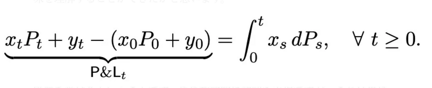
This equation is very important when considering the Rebalancing Portfolio. This formula is described in the paper as self financing strategy, and it shows that the P&L of the portfolio is affected by the price change of the riskey asset per minute. The equation is somewhat mathematically esoteric, but it can be thought of as a direct representation of the P&L that would be incurred if the Rebalancing Portfolio were constructed as described earlier: xt = 1, Pt = $4000, yt = 1000, x0 = 1, P0 = $1000, and y0 = 1000. In this case, xs = 1, dps = $3000, so 3000 is consistent with the previous example. In this case, since we are only dealing with a single point in time, the integral sign or even the Σ sign is too much to handle, but it is important to understand that this formula itself is only focusing on the P&Lof the Rebalancing Portfolio from time 0 to time t.
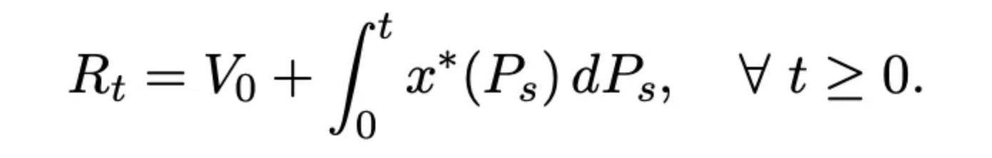
We could then construct a Rebalancing Portfolio by setting V0 with the same amount of assets as provided liquidity at the start as in the above equation. LVR can be defined as the difference between this Rebalancing Portfolio and the LP portfolio provided to DEX.